Particle filter localization on a VEX V5 robot

Why

An autonomous routine needs to know where the robot is on the field. Wheel odometry gives a pose, meaning an x, a y and a heading, but wheels slip and the error only grows over a run. The field has solid walls, and the robot carries distance sensors that point at them. The filter supports four (left, right, back and front); the test build ran with three, front disabled. The filter described here, a Monte Carlo localization filter (also called a particle filter), uses the walls to check the wheels. It is C++ on PROS, with LemLib supplying odometry and Eigen the maths.

I was team captain and lead programmer, and several of us worked on this code, so the page sticks to how the filter works. We ran it in our skills autonomous routine. The last section covers what was never measured.

The loop

The filter keeps 250 particles. Each is a guess at the full pose: x, y, heading and a weight. A background task runs the loop below every 20 ms.

Predict. LemLib reports how far the robot has moved since the last pass. Each particle moves by its own noisy copy of that movement, using the odometry motion model from Thrun, Burgard and Fox's Probabilistic Robotics (table 5.6). The model splits a move into a turn, a drive and a second turn, and the noise on each part grows with how much turning and driving there was. All four noise constants are 0.1, and I have not checked them against the drivetrain. Turning in place has zero drive distance, so the direction of travel is undefined, and the code sets the first turn to zero in that case.

sdRot1  = a1 * abs(rot1) + a2 * trans;
sdTrans = a3 * trans
        + a4 * (abs(rot1) + abs(rot2));
sdRot2  = a1 * abs(rot2) + a2 * trans;

// for each particle, N() drawn fresh each time
rot1Hat  = rot1  - N() * sdRot1;
transHat = trans - N() * sdTrans;
rot2Hat  = rot2  - N() * sdRot2;
p.x     += transHat * cos(p.theta + rot1Hat);
p.y     += transHat * sin(p.theta + rot1Hat);
p.theta += rot1Hat + rot2Hat;

Weigh. For each particle and each sensor, the filter works out which wall the beam would hit and how far away that is, which is ray-to-wall geometry on a square field with a half-width of 1.78308 m. It compares that with the real reading and scores the difference. A particle's weight is the product of the sensor scores, so it has to fit every sensor at once. The code gives each sensor a weight constant of 2.0. Particles that end up outside the field are re-injected at random positions, and if every weight collapses below 1e-6 that pass skips resampling.

Resample. Particles are copied in proportion to their weights with low-variance resampling: one random number sets a start, then 250 evenly spaced pointers walk along the cumulative weights. It only runs after the robot has moved 2 inches or 2 seconds have passed. After resampling all weights go back to one, and the noise from the next predict step spreads the copies out.

Estimate. The position is the mean of the particles' x and y, and the heading is a circular mean. The code can nudge LemLib's x and y a fraction (0.1 to 0.3) toward that estimate through blendMCLIntoOdometry, leaving heading alone.

Design choices

Heading belongs to each particle. The first version, on 27 January, kept only x and y per particle. Heading was added to each particle two days later, so the walls can now correct heading as well as position.

The score curve has a heavy tail. The error between predicted and real reading is divided by the sensor's uncertainty, set to 20 percent of the reading because distance sensors get less exact farther out. That goes through 0.3989 / (1 + 0.5942 x⁴) instead of a Gaussian. It has the same peak and much heavier tails: at four units of uncertainty it is about 19 times higher. A sensor that reads a game piece or another robot then lowers every particle's weight instead of zeroing most of them.

No return counts as far away. The distance sensor reports 9999 mm when nothing is in range. An earlier version skipped those readings. The current one treats them as a measurement of 3.0 m with 0.5 m of uncertainty, so particles that predict a wall close by are penalized.

w = 1;
for (sensor : sensors) {
  if (reading == 9999) { measured = 3.0; sigma = 0.5; }
  else { measured = reading; sigma = 0.2 * reading; }
  predicted = rayToWall(p, sensor);
  x = (predicted - measured) / sigma;
  w *= 0.3989 / (1 + 0.5942 * x*x*x*x);
}

Starting without a pose

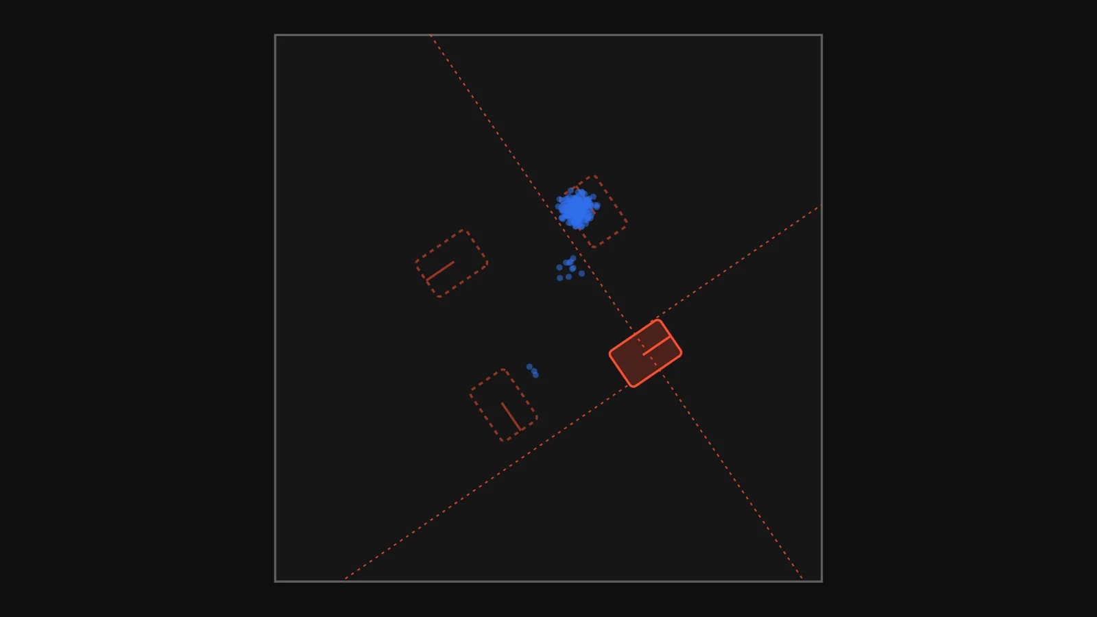
The field is square, so it looks the same after a quarter turn about its centre. Turn the robot, sensors and all, a quarter turn about the centre and every beam meets a wall at the same distance as before. Distance readings alone therefore have four equally good answers. If the particles start spread over the whole field, the cloud settles quickly on one of the four, and nothing in the readings says which.

I ran a small simulation to check this, shown below: the same weighting and resampling, a stationary robot and a uniform start. It resamples every step and uses small jitter in place of motion noise, so it is simpler than the robot's loop. The repository has no log of a lost start on the real robot, so the evidence is the geometry and this simulation.

It explains why the code has initializeAtPose, which seeds the particles within about 5 cm and 5 degrees of a given pose, and why the usage example in mcl_task.h calls it at the start of a routine.

Wall reset

distance_localizer.cpp holds a second way to use the same sensors, with no particles. It takes one set of readings and the robot's heading from the caller and works out the position directly. Each sensor picks the wall it most nearly faces, within 90 degrees, and the robot's position along that axis is the wall's position minus the reading, corrected for where the sensor is mounted. Readings for the same axis are averaged, weighted by each sensor's reported confidence. A reading is dropped if the sensor is missing, reads zero or 9000 mm and more, or meets the wall at too shallow an angle. Each sensor also has its own scale factor, between 0.979 and 0.987, applied to its readings. One use is after driving up to a wall: read the sensors, and the position follows.

This is instant and needs no history, but it needs a trusted heading and a clear view of two walls. The filter keeps working through a bad reading but needs a starting pose and some motion.

Status and limits

The repo shows a test build in late January 2026 with three sensors (back, left and right), a uniform start, a 5-inch forward test and a noise tuning change on 29 January. A logging task in that build printed the time, the odometry position, the filter's position and its spread ten times a second. The repository holds written test procedures: lift the robot and spin the wheels, push it without turning the wheels so only the sensors see the move, and turn it on the spot. It does not hold results from running them, so I cannot say how accurate the estimate is. We used the filter in our skills autonomous routine.

The sensor model knows only the four walls. Goals, game pieces and other robots show up as bad readings, and the heavy-tailed curve is the only thing softening them. The reported spread is a mean of squared distances floored at 0.05, which is about 22 cm root-mean-square at its smallest, so it says little about accuracy.

Next I would log its estimate against a tape-measured stopping point, and add an obstacle term so a game piece in front of a sensor stops counting as a wall.